


rm(list = ls())MODIS NRT Global Flood Product
LANCE MODIS Near Real Time (NRT) Global Flood Product
Overview
In this lesson, you will use R to take a closer look at the data from the LANCE MODIS Near Real Time (NRT) Global Flood Product, including learning about what are LANCE and MODIS, and the NRT Flood products available. You will then learn to select, download, and visualize one of the NRT Flood layers available. Lastly, we will use the NRT Flood data to calculate the area of each cropland type found in the flood zone, and plot the top ten results as a bar graph.
Coding Review
This lesson uses the R language and environment. R is a popular language used for statistical computing and graphics.
Learning Objectives
After completing this lesson, you should be able to:
Determine what NRT raster data is available by navigating the LANCE website.
Read a tile map and select a raster tile to download based on a point of interest.
Download near-real-time raster data using the application programming interfaces (APIs).
Preview the downloaded raster data.
Classify and place on a map the NRT flood spatial data to determine areas with unusual flooding.
Subset data, perform zonal statistics using spatial data, and graph analysis results.
Introduction
Atmospheric circulation, water evaporation, and their interactions with land surfaces can impact a region’s rainfall variability. For example, California’s winter is correlated with ocean evaporation near the West Coast and eastern North Pacific, and ocean evaporation is a strong factor in increased flooding in the region (Wei et al. 2016; University of California Museum of Paleontology (UCMP) 2022). Additionally, drought in the region is associated with high-pressure systems off the U.S. West Coast, with studies showing that high-pressure system are linked to the Pacific sea surface temperature anomalies, and exacerbated by high evaporation over land due to high temperatures (Wang et al. 2014; Hartmann 2015; Seager et al. 2015).
It is critical to understand the water cycle and how flooding events develop, particularly as climate change intensifies extreme weather events, the impacts of flooding can be a risk to human life and can disrupt infrastructure, agriculture, and natural habitats.
What are MODIS and LANCE?
MODIS
The Moderate Resolution Imaging Spectroradiometer (MODIS) is part of a NASA Earth Observing System (EOS). The satellite-based sensor system creates data products including land surface temperatures, land surface reflectance, radiances, clouds, aerosols, water vapor, active fire, snow cover, sea ice measurements, and other factor information . The MODIS NRT data includes the Flood product which we will explore in this lesson. The NRT Flood product is a daily ~250-meter resolution product showing flood and surface water detected from the twice-daily overpass of the MODIS optical sensors.
The satellite data is readily available shortly after it is acquired by the MODIS instrument on board the Terra and Aqua satellites. This space-based instrument distinguishes 36 spectral bands and groups of wavelengths in three different resolutions at 250 m, 500 m, and 1 km, all which helps map the extent of snow and ice caused by winter storms and frigid temperatures (Singh and Tiwari 2023). Initially, a water-detecting algorithm is applied to both MODIS observations (Terra and Aqua), however, cloud and terrain shadows are known to create false positives in the data.
MODIS is one of the most advanced systems that can produce earth-observing real time satellite data “designed to provide the maximum operational versatility and performance combined with long life. Most operations, including calibration, are performed under internal processor control in response to time-tagged commands from the spacecraft. The electronics are highly redundant, such that no single-point of failure can disable the data from more than one of the 490 MODIS detectors (Frazier 2015).”
The adoption of MODIS aimed to surpass barriers related to satellite data, such as cost, delivery timelines, limited formats, and the need for technical expertise. This transition led to the establishment of the Fire Information for Resource Management System (FIRMS) at the United Nations Food and Agriculture Organization (UN FAO), ensuring continuity in meeting NASA data-user needs (Lin et al. 2019; Davies, Justice, and Anderson 2010) .
LANCE
The Land, Atmosphere Near real-time Capability for EOS (LANCE) is a NASA initiative that provides near real-time access to satellite data, including MODIS. It allows users to access the latest data within a few hours of satellite overpass, enabling rapid responses to environmental events such as floods. Systems like LANCE highlight the importance of readily available data that can be easily consumed and analyzed through data analysis and data visualization for timely response. LANCE is particularly valuable for emergency response teams and researchers who require up-to-date information for monitoring and assessing natural disasters (Land 2024; Murphy et al. 2015).
LANCE reduces processing time, allowing for timely computation. Users access the data through platforms like Web Map Service (WMS) and Web Coverage Service (WCS), enabling visualization and analysis for informed decision-making. This NRT approach enhances the speed and accessibility of critical information on vegetation conditions (Zhang et al. 2022).
MODIS NRT Flood MCDWD Data Products
The MODIS/Aqua+Terra Global Flood Product L3 Near Real Time (NRT) 250m Global Flood Product (MCDWD_L3_NRT) (Release 1) provides daily maps of flooding globally. The product is provided over 3 compositing periods (1-day, 2-day, and 3-day) to minimize the impact of clouds and more rigorously identify flood water. The best composite will depend on the cloudiness of a particular event (Lin et al. 2019).
Data Information
The main landing pages for the MODIS NRT Global Flood Product:
The MODIS/Terra+Aqua Combined MODIS Water Detection (MCDWD) algorithm is tailor-made for detecting water bodies using MODIS data obtained from both the Terra and Aqua satellites. This algorithm employs various bands and spectral information to effectively identify and categorize water bodies. This enhances the accuracy and reliability of the flood product generated (Slayback 2023). To minimize errors, the product is generated with three different compositing periods (1-day, 2-day, and 3-day) to compare results and decide which product has better coverage for the event. Further, then product differentiates floods from expected surface water through the use of the MODIS Land Water Mask (MOD44W), which uses a decision tree classifier trained with MODIS data to produce a global water mask (Carroll et al. 2016).
The MODIS Near Real-Time (NRT) Flood dataset offers multiple products, each accompanied by corresponding layers. The specific layers depend on the temporal aggregation:
MCDWD_F1_L3_NRT (1-Day product) This product type is the most basic level and provides binary information about water occurrence. Pixels are classified as either containing water or not, offering a simple way to identify flooded areas.
MCDWD_F1CS_L3_NRT (1-Day CS): F1CS has a cloud shadow mask applied on the version of the MCDWD_F1_L3_NRT product. A cloud shadow mask identifies areas that are cloud or shadow of cloud and categorizes them separately. This layer is produced because sometimes cloud-shadows can produce false positives in the data product. Thus, the cloud shadow mask can improve some analysis, however, the cloud mask can also produce errors and remove real water (Rayne 2024). See section 3.4.3 in the MODIS User Guide.
MCDWD_F2_L3_NRT (2-Day): F2 provides additional information by categorizing water occurrences into three categories: no water, low-confidence water, and high-confidence water. This classification allows for a more nuanced understanding of the extent of the flood and its associated confidence levels.
MCDWD_F3_L3_NRT (3-Day): The F3 product, based on the MCDWD (MODIS/Terra+Aqua Combined MODIS Water Detection) is an algorithm that further refines flood mapping by adding additional spectral information. These results create a more accurate representation of water bodies and flooded areas (Slayback 2023).
Exploring the Data
For this exercise, we will be using the MCDWD L3 F3 product: LANCE NRT Flood
If in 2i2c, clear objects from the current workspace:
First, install and load the R packages required for this exercise:
#List the necessary packages and then check if they are installed
packages_to_check <- c("stars", "httr", "jsonlite", "tmap", "basemaps", "sp", "sf", "ggplot2")
# Check and install packages
for (package_name in packages_to_check) {
if (!package_name %in% rownames(installed.packages())) {
install.packages(package_name)
cat(paste("Package", package_name, "installed.\n"))
} else {
cat(paste("Package", package_name, "is already installed.\n"))
}
library(package_name, character.only = TRUE)
}Package stars is already installed.
Package httr is already installed.
Package jsonlite is already installed.
Package tmap is already installed.
Package basemaps is already installed.
Package sp is already installed.
Package sf is already installed.
Package ggplot2 is already installed.#in case tmap does not install
#remotes::install_github('r-tmap/tmap')Step 2, check what days are available for the MCDWD L3 F3 product by going to this link: LANCE NRT Primary Server or Secondary. Note: you must have a NASA Earthdata Account.
Based on availability, edit the year_day variable YYYY-DD. Example: ‘2022-01’
#add the year and date you want to search for (YYYY-DD, 2022-01)
year_day <- '2024-163'Determine tiles of interest:
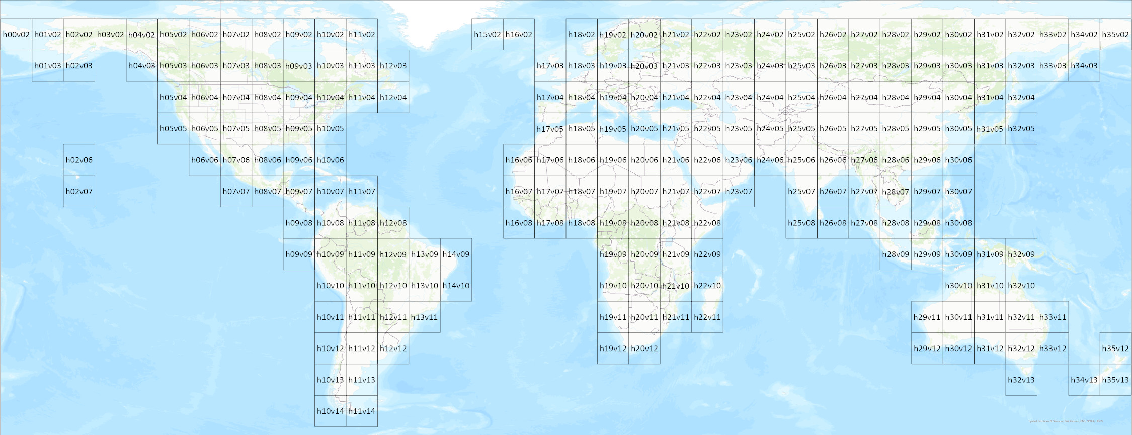

Based on availability, edit the tile_code variable:
#add tile code from the map above (written as h00v00)
tile_code <- 'h05v05'This is the NRT Flood F3 (MCDWD_L3_F3) API URL:
# Primary Server
API_URL <- paste0('https://nrt3.modaps.eosdis.nasa.gov/api/v2/content/details?products=MCDWD_L3_F3_NRT&archiveSets=61&temporalRanges=')
# if the primary server is down, the secondary server may be available:
#API_URL <- paste0('https://nrt4.modaps.eosdis.nasa.gov/api/v2/content/details?products=MCDWD_L3_F3_NRT&archiveSets=61&temporalRanges=')We can combine the API URL above with the year_day provided and print the available datasets:
#pasting together URL and year_day
url <- paste0(API_URL, year_day)
print(url)[1] "https://nrt3.modaps.eosdis.nasa.gov/api/v2/content/details?products=MCDWD_L3_F3_NRT&archiveSets=61&temporalRanges=2024-163"Loading the Data
NASA Earthdata requires a NASA username and token. Go here to learn How to generate a User Token.
Once you have generated a User Token, you can access NASA Earthdata using the GET function (Wilson 2024). Replace USER_TOKEN with the token you generated:
token <- "USER_TOKEN"Combine the token with "Bearer" into a single text string.
api_key <- paste("Bearer", token)This code is for use on a local computer, not 2i2. Use to protect your token locally.
# Define headers (include your token)
headers <- c(Authorization = api_key)
# Make GET request
response_content <- GET(url, add_headers(.headers=headers))Check the response status from the GET function:
response_contentResponse [https://nrt3.modaps.eosdis.nasa.gov/api/v2/content/details?products=MCDWD_L3_F3_NRT&archiveSets=61&temporalRanges=2024-163]
Date: 2024-07-02 18:52
Status: 200
Content-Type: application/json;charset=UTF-8
Size: 145 kBOut of the response from the server, we’ll check if the response was a success with if (http_status(response)$category == "Success"). If this statement is true, then the content will be assigned to the variable data in JSON format, which is then parsed to a data frame using data_parsed <- jsonlite::fromJSON(data). The data frame contains data_parsed$content, a column with content. We filter the content by tile code using the command content_items <- data_parsed$content[grepl(tile_code, data_parsed$content$name, ignore.case = TRUE), ] and add the results to a data frame.
if (http_status(response_content)$category == "Success") {
# Read the JSON content into a data frame
response_content <- content(response_content, as = "parsed", simplifyVector = TRUE)
response_content <- response_content$content
} else {
print("Request failed with status code", http_status(response_content)$status_code)
}
names(response_content) [1] "archiveSets" "cksum" "collections" "dataDay"
[5] "downloadsLink" "fileId" "md5sum" "mtime"
[9] "name" "products" "resourceType" "self"
[13] "size" Search the Data Frame and subset the rows that contain tile_code in the downloadsLink column.
# Subset rows where the downloadsLink column contains the tile code
response_content <- response_content[grepl(tile_code, response_content$downloadsLink), ]
response_content archiveSets cksum collections dataDay
104 61 3613949109 modis-nrt-c6.1 2024-163 = 2024-06-11
downloadsLink
104 https://nrt3.modaps.eosdis.nasa.gov/api/v2/content/archives/MCDWD_L3_F3_NRT.A2024163.h05v05.061.tif
fileId md5sum mtime
104 2269072539 98f4a6d1cba74a32c3869643d19a2f60 1718158322
name products resourceType
104 MCDWD_L3_F3_NRT.A2024163.h05v05.061.tif MCDWD_L3_F3_NRT File
self size
104 /api/v2/content/details/MCDWD_L3_F3_NRT.A2024163.h05v05.061.tif 868848If there is only 1 row, select the string ‘downloadsLink’ column:
response_content <- response_content$downloadsLink
print(response_content)[1] "https://nrt3.modaps.eosdis.nasa.gov/api/v2/content/archives/MCDWD_L3_F3_NRT.A2024163.h05v05.061.tif"Read the Data
Use the read_stars() function from the stars R Library to read the geoTiff raster. The raster is assigned to the raster_df variable. This is a web-derived layer that is in the Geographic Coordinate System (GCS) WGS84 - World Geodetic System 1984 EPSG:4326 (EPSG number 4326). We can assign the Coordinate Reference System (CRS) to the stars object:
#read the raster data from the download_link
raster_df <- read_stars(response_content)
#Set a CRS for the stars object based on the data documentation
st_crs(raster_df) <- st_crs(4326)Visualizing NRT Flood Data
Plot the raster to quickly view it. downsample allows faster rendering for viewing:
plot(raster_df, downsample=30)
Create NRT Flood Plot with Classification
Refer to the MODIS NRT Global Flood Product User Guide for more information.
NRT Flood data has 5 classifications:
| Code | Definition |
|---|---|
| 0 | No Water |
| 1 | Surface Water |
| 2 | Recurring flood4 |
| 3 | Flood (unusual) |
| 255 | Insufficient data |
To view the data in this classification, we’ll need to create a classified legend; however, the NRT Flood data is stored in decimal numbers (known as floating-point). Class breaks allow us to group together data depending on the values. Create classification breaks that divide the data using the breaks listed below and their corresponding colors and labels. Finally, add a title for the plot that includes the year and day, year_day, and the tile_code:
#class_breaks for the table plot categorization
class_breaks <- c( 0, 1, 2, 3, Inf)
#colors for the plot breaks
colors <- c( "gray", "blue", "yellow", "red")
#labels for the plot breaks
labels = c("0: No Water", "1: Surface Water", "2: Recurring flood", "3: Flood (unusual)")
title = paste("Near Real-Time Flood F3", year_day, tile_code)Generate a basemap from Esri Imagery
The basemap_stars() function from the stars package allows us to access Esri imagery layers. To generate a basemap that shows the location of our raster, we must first define the bounding box with the raster_df. Choose “world_imagery” as our background and assign it to the object bm_m. The st_rgb function combines the basemap RGB image into a single file. Finally, st_transform transforms the CRS into WGS84.
#define basemap using a the raster as a bounding box
bm_m <- basemaps::basemap_stars(raster_df, map_service = "esri", map_type = "world_imagery")Loading basemap 'world_imagery' from map service 'esri'...#The `st_rgb` function lets us turn the RGB stars item into a single image
bm_m <- st_rgb(bm_m)
#transform the CRS of the basemap to match the flood raster
bm_m <- st_transform(bm_m, 4326)Plot basemap and NRT Flood data
Generate a plot from the tmap library using the tm_shape() function. We will plot the basemap and the raster_df items in one plot.
## tmap mode set to "plot"
tmap_mode("plot")
## tmap mode can also be set to "view"
#tmap_mode("view")
#create an object that plots the basemap and the NRT flood raster
#with the tmap library, call the tm_shape() function for the basemap
tm_plot <- tmap_options(max.raster = c(plot = 50000, view = 50000))+
tm_shape(bm_m)+
#the basemap bm_m is treated as a raster
tm_raster()+
#create a new tmap shape for the NRT flood raster with a style as "cat," meaning categorical.
tm_shape(raster_df, style="cat")+
#add the classification styling to the raster including colors, title, class breaks, and labels
tm_raster( palette = c(colors),
title = title,
breaks = class_breaks,
labels = labels )+
#style the plot
tm_layout(legend.outside = TRUE) +
tm_graticules(lines=FALSE)
#view Plot
tm_plot
To observe a location more closely, we can create a new bounding box using latitude and longitude values, clip the data, and replot on a map. First, select from the map four corners in degrees that include North/South and East/West information. We use these coordinates to create a matrix of points representing four corners; the four corners are then used to create a bounding box. The corners are first placed in the GCS WGS84 to match our raster.
# Define the NWES coordinates
north <- 40 #negative values are used for South
south <- 36 #negative values are used for South
west <- -124 #negative numbers are used for West
east <- -120 #negative numbers are used for West
# Create a bounding box
bbox_subset <- st_bbox(c(xmin = west, ymin = south, xmax = east, ymax = north), crs = 4326)We redo the same process as above to plot the data with a basemap but with a different bounding box:
#generate a new basemap
bm_m <- basemaps::basemap_stars(bbox_subset, map_service = "esri", map_type = "world_imagery")Loading basemap 'world_imagery' from map service 'esri'...#combine RGB bands of the bsemap
bm_m <- stars::st_rgb(bm_m)
#transform to CRS 4326
bm_m <- sf::st_transform(bm_m, 4326)## tmap mode set to "plot"
tmap_mode("plot")
## tmap mode can also be set to "view"
#tmap_mode("view")
#create an object that plots the basemap and the NRT flood raster
#with the tmap library, call the tm_shape() function for the basemap
tm_plot <- tmap_options(max.raster = c(plot = 50000, view = 50000))+
tm_shape(bm_m, raster.downsample=TRUE)+
tm_raster()+
#create a new tmap shape for the NRT flood raster with style as "cat," meaning categorical.
tm_shape(raster_df, style="cat", raster.downsample=TRUE)+
#add the classification styling to the raster
tm_raster( palette = c(colors),
title = title,
breaks = class_breaks,
labels = labels )+
#style the plot
tm_layout(legend.outside = TRUE) +
tm_graticules(lines=FALSE)
#View the plot:
tm_plot
Zonal Statistics of Flood Zones
The NRT flood data can be compared to the Cropland Data Layer (CDL), which provides agricultural categories based on the Farm Service Agency (FSA) Common Land Unit (CLU) Program and is produced by the U.S. Department of Agriculture National Agricultural Statistics Service (NASS)(USDA-NASS 2023).
To quantify how many acres of each cropland may be affected by the flooding identified in the NRT Flood data, we can explore the dataset by using the Cropland Collaborative Research Outcomes System (CroplandCROS), and we can download the data from the NASS website
Download the latest CDL year of data available from the NASS website.
For this part of the exercise, we will use the package stars, discussed in the previous lesson, and the function read_stars() to read the CDL raster as a stars object.
#Read CDL GeoTIFF
cdl<- read_stars("data/2022_30m_cdls.tif")
#plot the raster and downsample by 100 as the resolution of the raster is high
plot(cdl, downsample=100)
This raster is provided with a 30-meter resolution for the entire contiguous U.S.! Additionally, the coordinate reference system(CRS) is the North American Datum of 1983 (NAD83) / Albers Conical Equal Area (AEA) EPSG:5070 projection. We can subset a stars objects with other stars objects if they have the same CRS. We will first subset the NRT Flood raster and project the data into the same CRS as the CDL raster. We can subset this raster with the NRT flood raster, but we must first crop it with the bounding box bbox_subsetwe created previously. We will then use the warp() function to change the raster from the CRS WGS84 EPSG:4326 to NAD83 EPSG:5070:
#subset the NRT Floor raster with the bounding box
raster_df <- raster_df[bbox_subset]
#warp the raster NRT flood raster to match the CDL raster CRS.
raster_df <- st_warp(raster_df, crs=5070, use_gdal=FALSE,method = "near")
#subset CDL raster with the subset NRT flood raster
cdl <- cdl[raster_df]
#because of the high resolution, a stars proxy object was made
#make a stars object from a stars proxy object to directly read the data
cdl <- st_as_stars(cdl)
#plot the resulting CDL subset
plot(cdl, downsample=100)
We are only interested in the areas that are showing as category 3, Flooded (unusual); therefore, we want to exclude other variables. We can do this by setting variables that are not 3 as NA. Once we have only the flooded areas from the NRT Flood data, we can subset the CDL data.
#set variables as NA that do NOT equal 3
raster_df[raster_df != 3] <- NA
#subset the CDL raster where unusual flooding occurred
cdl <- cdl[raster_df==3] The CDL FAQ Webpage lists the categorization, including non-agricultural categories which we can remove from the analysis:
Non-Agricultural Categories
| Categorization Code | Land cover |
|---|---|
| “111” | Open water |
| “112” | Perennial Ice/snow |
| “121” | Developed/Open space |
| “122” | Developed/Low Intensity |
| “123” | Developed/Med Intensity |
| “124” | Developed/High Intensity |
| “131” | Barren |
| “141” | Deciduous Forest |
| “142” | Evergreen Forest |
| “143” | Mixed Forest |
| “152” | Shrubland |
| “176” | Grassland/Pasture |
| “190” | Woody Wetlands |
| “195” | Herbaceous Wetlands |
`
#list of non-agricultural Categories
nonag_cat <- list("Open Water", "Perennial Ice/Snow", "Developed/Open Space", "Developed/Low Intensity", "Developed/Med Intensity","Developed/High Intensity", "Barren", "Deciduous Forest", "Evergreen Forest","Mixed Forest","Shrubland","Grassland/Pasture","Woody Wetlands", "Herbaceous Wetlands")
#exclude non-agricultural categories
for (category in nonag_cat){
cdl[cdl == category ] <- NA
}Next, we can create a table out of the remaining CDL raster data, but we first have to extract it from the stars object and convert it to a matrix. The matrix can then be converted to a table and sorted.
# Convert the stars object to a matrix
cdl <- as.matrix(cdl)
# Count the number of pixels for each category
cdl <- table(cdl)
#Sort the `cdl_counts` table by descending order.
cdl<- sort(cdl, decreasing = TRUE)Select the top 10 CDL categories counted.
top_10 <- cdl[1:10]
#print top 10
print(top_10)cdl
Almonds Fallow/Idle Cropland Grapes
8525 4910 3832
Walnuts Alfalfa Winter Wheat
2976 2690 2103
Pistachios Rice Tomatoes
2086 1398 1364
Other Hay/Non Alfalfa
1164 Turn the top 10 table into a dataframe. This will allow us to more easily handle the dataframe table and data.
dataplot <- as.data.frame(top_10)According to the NASS CDL data documentation, each of the CDL’s pixels represents 30 square meters. Additionally, a hectare is 10,000 meters. We can calculate the hectares of each CDL category by first multiplying the count of each category by 30 and dividing by 10,000.
# Calculate the area for each row
dataplot$area <- dataplot$Freq * 30 / 10000Once the area is calculated, we can plot a bar graph to compare the top 10 CDL Categories found in the NRT Flood zone.
#create new title for plot
title = paste("Hectares of NASS CDL Cropland Category under flood, \nday", year_day, "in tile", tile_code)
# Find the max value in the table for a dynamic axis plot
max_value <- max(dataplot$area) +3
# use ggplot to plot the dataplot table with area
# in x axis and category name in the y axis
plt <- ggplot(dataplot, aes(x = area, y = cdl)) +
geom_bar(stat = "identity", fill = "skyblue") + # adjust the height and color
geom_vline(xintercept = seq(0, max_value, by = 1),
color = "gray", linetype = "dashed") + #create guide lines
labs(title = title, x = "Hectares (ha)", y = "Categories") + #add labels to plot
theme_minimal() + #set theme
theme(axis.line = element_line(size = 1), # Adjust size of axis lines
axis.ticks = element_line(size = 1),# Adjust size of axis ticks
panel.grid.major = element_blank(), # Remove major gridlines
panel.grid.minor = element_blank(),# Remove minor gridlines
plot.background = element_rect(fill = "white"),# Set plot background color
panel.background = element_rect(fill = "white"),# Set panel background color
panel.border = element_rect(color = "black", fill = NA)) + # Set panel border
geom_text(aes(label = round(area,1)), color = "black") +
xlim(0, max_value) # Adjust x-axis limits # Adjust size of text labels
plt
The graph above shows the hectares (ha) of land that were calculated using the NRT Flood data and the CDL cropland data within the bounding box we generated. We did this by selecting the area with abounding box, then subsetting the CDL data to areas that are labeled as “Unusually Flooded” by the NRT Flood data on a particular day, and counting the number of pixels by CDL category. With the count of pixels and the resolution of the CDL dataset, we calculated the total area flooded for each category in ha.
Congratulations! We were able to download and explore NASA NRT Flood data to pick an area of interest in the contiguous U.S. and determine how much cropland may be affect by floods. Now you should be able to:
Navigate the LANCE data website and determine what data is available.
Select a tile and date to download NRT data.
Create a GET HTTP request to download near-real-time data.
Plot on a map and classify raster data to determine areas with unusual flooding.
Use NRT Flood data to subset cropland classification data, perform zonal statistics, and graph results.
Lesson 3
In this lesson, we explored the LANCE MODIS Near-Rear-Time (NRT) Flood dataset. In our next lesson, we will think of water at the local level and focus on New York State School Drinking Water data.
Lesson 3: New York State School Water Quality: Exposure to Lead
References
Carroll, M. L., C. M. DiMiceli, J. R. G. Townshend, R. A. Sohlberg, A. I. Elders, S. Devadiga, A. M. Sayer, and R. C. Levy. 2016. “Development of an Operational Land Water Mask for MODIS Collection 6, and Influence on Downstream Data Products.” International Journal of Digital Earth 10 (2): 207–18. https://doi.org/10.1080/17538947.2016.1232756.
Davies, Diane, Chris Justice, and Gretchen-Cook Anderson. 2010. “NASA Global Fire Information System Adopted by UN Food and Agriculture Organization.” The Earth Observer 22 (6). https://eospso.nasa.gov/sites/default/files/eo_pdfs/Nov_Dec10.pdf.
Frazier, Shannell. 2015. “MODIES - Door Assemblies - Earth View Door.” 2015. https://modis.gsfc.nasa.gov/about/earthviewdoor.php.
Hartmann, Dennis L. 2015. “Pacific Sea Surface Temperature and the Winter of 2014.” Geophysical Research Letters 42 (6): 1894–1902. https://doi.org/10.1002/2015gl063083.
Land, Atmosphere Near real-time Capability for EO (LANCE). 2024. “About LANCE.” January 11, 2024. https://www.earthdata.nasa.gov/learn/find-data/near-real-time/about-lance.
Lin, Li, Liping Di, Junmei Tang, Eugene Yu, Chen Zhang, Md. Rahman, Ranjay Shrestha, and Lingjun Kang. 2019. “Improvement and Validation of NASA/MODIS NRT Global Flood Mapping.” Remote Sensing 11 (2): 205. https://doi.org/10.3390/rs11020205.
Murphy, Kevin J., Diane K. Davies, Karen Michael, Christopher O. Justice, Jeffrey E. Schmaltz, Ryan Boller, Bruce D. McLemore, Feng Ding, Bruce Vollmer, and Min M. Wong. 2015. “LANCE, NASA’s Land, Atmosphere Near Real-Time Capability for EOS.” In, 113–27. Springer New York. https://doi.org/10.1007/978-1-4939-2602-2_8.
Rayne, Nyssa. 2024. “Moderate Resolution Imaging Spectroradiometer.” 2024. https://terra.nasa.gov/about/terra-instruments/modis.
Seager, Richard, Martin Hoerling, Siegfried Schubert, Hailan Wang, Bradfield Lyon, Arun Kumar, Jennifer Nakamura, and Naomi Henderson. 2015. “Causes of the 201114 California Drought*.” Journal of Climate 28 (18): 6997–7024. https://doi.org/10.1175/jcli-d-14-00860.1.
Singh, Abhay Kumar, and Shani Tiwari. 2023. Atmospheric Remote Sensing. Elsevier. https://doi.org/10.1016/c2021-0-02005-8.
Slayback, D. 2023. “Modis NRT Global Flood Product - Earthdata.” https://www.earthdata.nasa.gov/s3fs-public/2023-01/MCDWD_UserGuide_RevC.pdf.
University of California Museum of Paleontology (UCMP). 2022. “Atmospheric Circulation. Understanding Global Change.” March 8, 2022. https://ugc.berkeley.edu/background-content/atmospheric-circulation/.
USDA-NASS. 2023. “USDA National Agricultural Statistics Service Cropland Data Layer.” Washington, DC. 2023. https://croplandcros.scinet.usda.gov/.
Wang, S.-Y., Lawrence Hipps, Robert R Gillies, and Jin-Ho Yoon. 2014. “Probable Causes of the Abnormal Ridge Accompanying the 20132014 California Drought: ENSO Precursor and Anthropogenic Warming Footprint.” Geophysical Research Letters 41 (9): 3220–26. https://doi.org/10.1002/2014gl059748.
Wei, Jiangfeng, Qinjian Jin, Zong-Liang Yang, and Paul A. Dirmeyer. 2016. “Role of Ocean Evaporation in California Droughts and Floods.” Geophysical Research Letters 43 (12): 6554–62. https://doi.org/10.1002/2016gl069386.
Wilson, James. 2024. “NASA API Overview.” November 30, 2024. https://github.com/wilsjame/how-to-nasa?tab=readme-ov-file.
Zhang, Chen, Zhengwei Yang, Liping Di, Eugene G. Yu, Bei Zhang, Weiguo Han, Li Lin, and Liying Guo. 2022. “Near-Real-Time MODIS-Derived Vegetation Index Data Products and Online Services for CONUS Based on NASA LANCE.” Scientific Data 9 (1). https://doi.org/10.1038/s41597-022-01565-2.