WSIM-GLDAS
Acquisition, Exploration and Integration with Water Security Indicator Model - Global Land Data Assimilation System (WSIM-GLDAS).
In this comprehensive lesson, you will embark on an immersive journey that combines advanced data acquisition, pre-processing, and exploration of vital water security data. Specifically, you will retrieve the Water Security Indicator Model - Global Land Data Assimilation System (WSIM-GLDAS) dataset, available from NASA’s Socioeconomic Data and Applications Center (SEDAC). This dataset provides crucial insights into water anomalies, such as droughts and floods, and will serve as the foundation for your analysis.
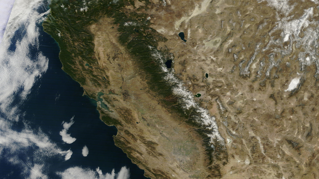
This true color satellite image of California illustrates regions experiencing water stress such as droughts. Visual representations like this are essential for understanding the spatial distribution of water security risks and guiding decision-making processes to manage limited freshwater resources. [11]
As you progress through this lesson, you will be guided step by step through several pre-processing tasks designed to help you make sense of this complex data. You will learn not only how to handle and subset the WSIM-GLDAS dataset but also how to enhance its value by integrating it with other globally recognized datasets. In particular, you will incorporate the geoBoundaries dataset, which offers global administrative boundary data, and the Gridded Population of the World dataset, a vital resource for understanding how human populations are affected by water anomalies.
Through the lesson, you’ll engage in a series of data manipulations and visualizations, gaining practical skills in handling large-scale geospatial data. These advanced visualizations will empower you to reveal patterns in precipitation deficits and surpluses, providing a clearer understanding of how water-related events impact specific regions. Ultimately, by the end of the lesson, you’ll have a complete workflow in place to retrieve, process, and visualize complex data, arming you with the tools to explore critical water security issues affecting communities around the globe.
Learning Objectives
By the end of this lesson, you will have developed a solid understanding of the technical and analytical skills needed to work with complex datasets in the field of water security. You will have gained the ability to:
Retrieve WSIM-GLDAS Data. Confidently access the WSIM-GLDAS dataset from the NASA SEDAC website, ensuring you can efficiently acquire the necessary data for analysis.
Access Administrative Boundaries. Use the geoBoundaries API to retrieve up-to-date global administrative boundary data, allowing you to contextualize the WSIM-GLDAS dataset within specific regional borders.
Subset WSIM-GLDAS Data. Learn how to filter and subset the WSIM-GLDAS data for specific regions and time periods, enabling you to focus on areas of particular interest in your analysis.
Visualize Geospatial Data. Create insightful geospatial visualizations that highlight patterns of precipitation deficits, helping you to communicate complex findings with clarity and precision.
Save Pre-Processed Data. Export your pre-processed NetCDF-formatted files to disk, giving you the ability to save and share your refined datasets for future use or collaboration.
Explore Data Visually. Master advanced data visualization techniques, including the creation of histograms, choropleths, and time series maps, to explore patterns and trends within the dataset.
Integrate Population Data. Combine the WSIM-GLDAS data with Gridded Population of the World data to analyze how water anomalies intersect with population distribution, providing valuable insights into the human impacts of water security issues.
Summarize Data with Zonal Statistics. Utilize zonal statistics to summarize the WSIM-GLDAS and population raster data, providing an analytical overview of how water shortages or surpluses affect specific regions and communities.
Through these objectives, you will not only gain proficiency in handling complex geospatial data but also develop a deeper understanding of how these datasets can be leveraged to solve real-world challenges, particularly in the realm of water security and population impacts.
Introduction
The Water cycle, also known as the Hydrologic cycle, refers to the continuous movement and circulation of water across, above, and below the Earth’s surface. It is a fundamental process that sustains life, ensuring that water is recycled and made available through precipitation, evaporation, and condensation (NOAA, 2019 [1]). However, human activities in recent decades — such as the emission of greenhouse gases, land-use alterations, the construction of dams and reservoirs, and the extraction of groundwater — have increasingly disrupted the natural flow of this cycle (IPCC, 2023 [2]). These anthropogenic influences have had significant and far-reaching consequences on various processes tied to oceans, groundwater systems, and land surfaces. As a result, extreme events like droughts and floods are becoming more frequent and intense (Zhou, 2016 [3]).
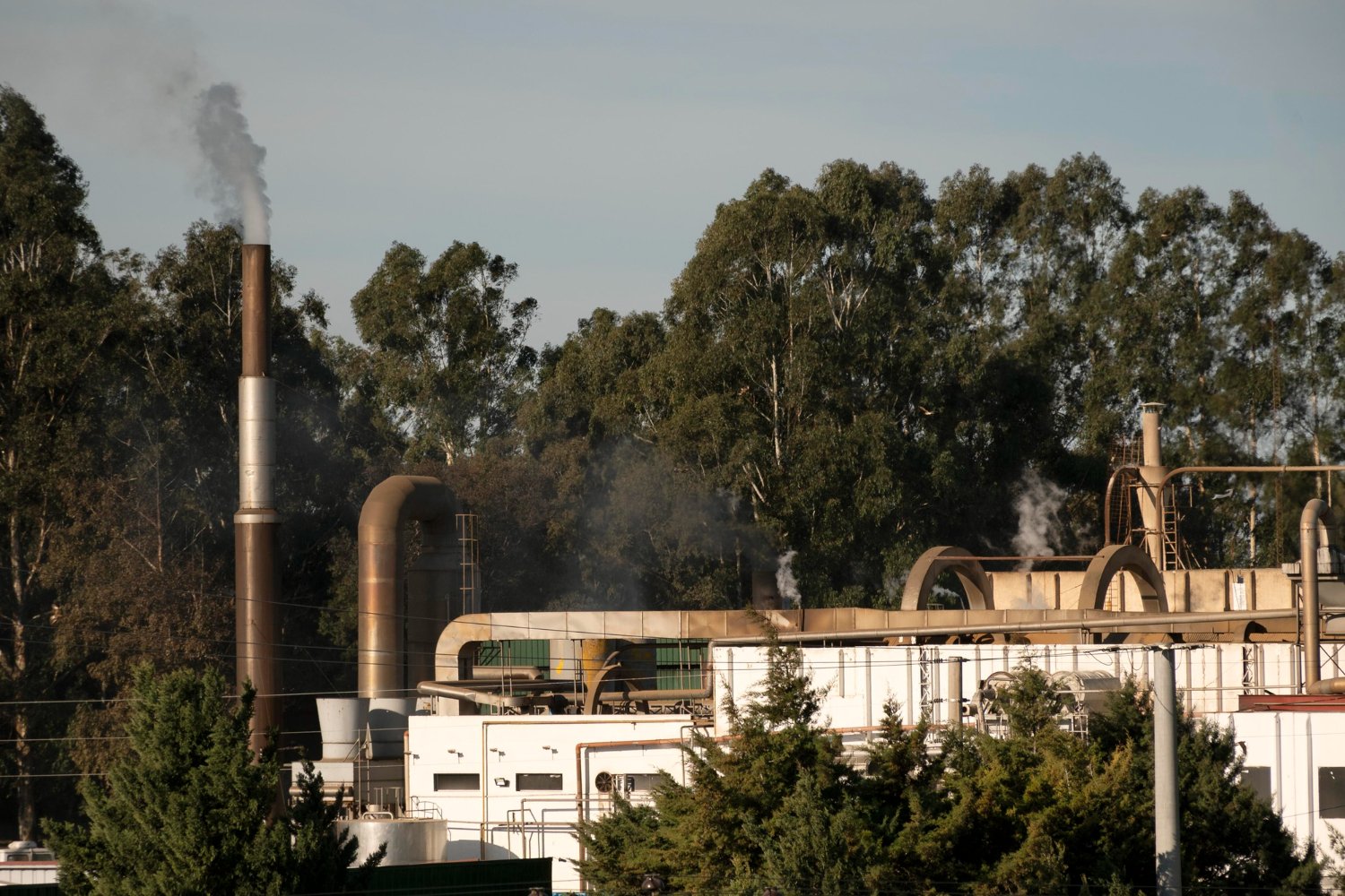
Impact of Human Activities on the Water Cycle. Human activities such as greenhouse gas emissions, deforestation, and dam construction are altering the natural flow of the water cycle, leading to environmental imbalances.
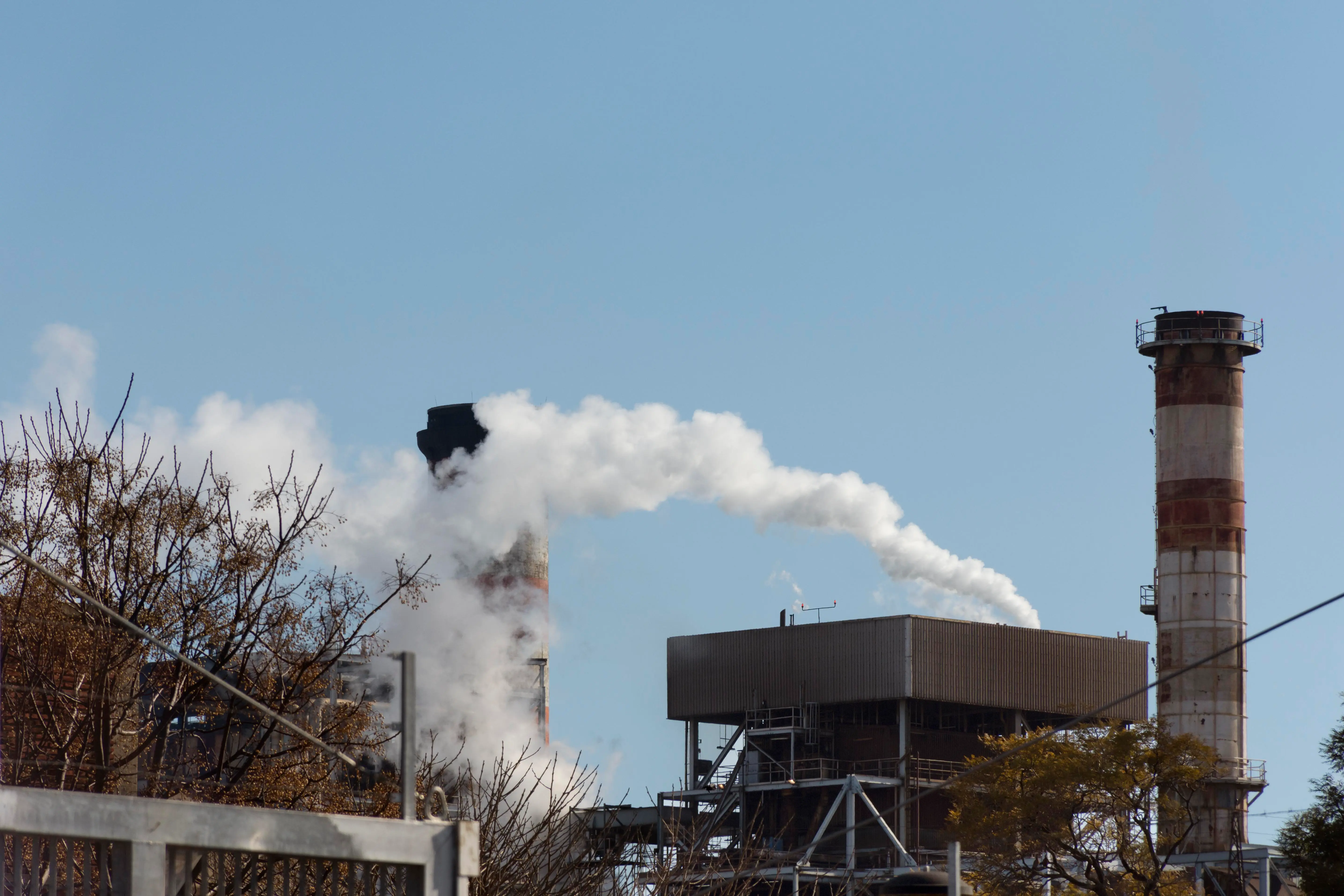
Impact of Human Activities on the Water Cycle. Human activities such as greenhouse gas emissions, deforestation, and dam construction are altering the natural flow of the water cycle, leading to environmental imbalances.
Drought, which occurs when precipitation deficits persist over time, is characterized by prolonged dry periods that lead to severe water shortages. The cascading effects of drought are felt across ecosystems, agriculture, and human communities, often creating feedback loops that exacerbate environmental stresses (Rodgers, 2023 [4]). For instance, California is notorious for recurrent droughts, but prolonged dry spells, coupled with sustained high temperatures, severely reduced the replenishment of fresh water to key water bodies like the Klamath River. From 2003 to 2014, the state experienced extreme water shortages that had devastating effects. These shortages significantly impacted California’s Central Valley, a vital agricultural region responsible for producing 80% of the world’s almonds. The droughts also caused ecological distress by triggering declines in Chinook salmon populations, as the lack of fresh water led to heat stress and disease outbreaks among the fish, affecting the Klamath basin tribal groups, who rely heavily on these salmon for sustenance (Guillen, 2002 [5]; Bland, 2014 [6]).
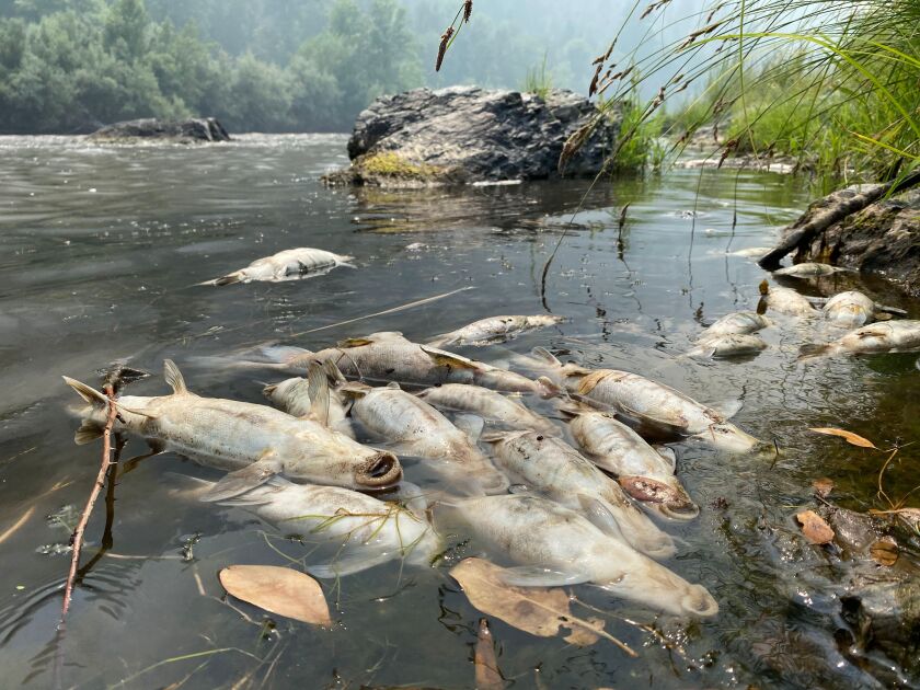
Indigenous Communities and Water Resources. The Klamath basin tribal groups depend on the Chinook salmon for their livelihood, but water shortages and environmental stress have led to a significant decline in salmon populations. [10]
To better understand and quantify such changes in water availability and their implications, datasets like the Water Security (WSIM-GLDAS) Monthly Grids, v1 (1948 - 2014) are invaluable. This particular dataset offers detailed insights into freshwater surpluses and deficits across the globe, tracking them monthly over a 66-year period from January 1948 to December 2014 (ISciences & CIESIN-Columbia University, 2022b [7]).
The WSIM-GLDAS dataset organizes its data by thematic variables such as temperature, runoff, soil moisture, precipitation, and evapotranspiration, as well as temporal aggregation periods (e.g., 1-month, 3-month, 6-month, and 12-month intervals). This structure allows for comprehensive exploration of water-related anomalies across various timescales. The data files, stored in NetCDF (.nc) format, contain time-dimensioned raster layers, each representing one of the 804 months in the dataset. Some variables even contain multiple attributes with their own time series. It is important to note that because the dataset is vast and consists of multiple layers, downloading and handling the files can be resource-intensive, possibly leading to memory issues on some computers.
This dataset represents what is known as “Big Data”, requiring advanced tools and techniques to analyze and draw meaningful conclusions from. By working with this dataset, students and researchers will gain practical experience dealing with complex, large-scale data, while also exploring critical water security issues at a global level.
Acquiring the Data
For this lesson, we will work with the WSIM-GLDAS dataset focusing on the Composite Anomaly Twelve-Month Return Period NetCDF file. This file includes water deficit, surplus, and composite anomaly variables, each with a 12-month integration period. The integration period refers to the timeframe over which anomaly values are averaged. In this case, the 12-month integration averages water-related anomalies like droughts and floods over a year, providing a high-level overview of water deficits, surpluses, and combined anomalies. This helps in understanding yearly trends, and once we’ve identified key time periods of interest, we can refine our analysis using the 3-months or 1-month integration periods.
We’ll start by downloading the file directly from the SEDAC website. The dataset documentation highlights the composite variables as essential elements of WSIM-GLDAS, which integrate the return periods of multiple water-related parameters into composite indices of overall water surpluses and deficits (ISciences & CIESIN-Columbia University, 2022a [7]). These composite anomaly files provide data in terms of return periods, indicating how often anomalies such as droughts or floods occur. For example, a deficit return period of 25 suggests a drought so severe that it would only occur once every 25 years.
Downloading Data
Visit the SEDAC website.
You can navigate through themes, datasets, or collections on the platform. For this exercise, use the search bar to look up “water security wsim.”
Locate and select the Water Security (WSIM-GLDAS) Monthly Grids, v1 (1948-2014) dataset. Take a few moments to review the dataset’s overview and documentation.
When you’re ready, go to the Data Download tab. You’ll need to sign in using your NASA EarthData account.
Once logged in, find the Composite Class and select the Variable Composite Anomaly Twelve-Month Return Period for download.
Reading the Data
After downloading the WSIM-GLDAS file to your local machine, the next step is to prepare your R environment by installing and loading the necessary R packages. This is an essential part of ensuring your system is ready to handle the data processing efficiently.
install.packages('stars')
install.packages('terra')
install.packages('sf')
install.packages('cubelayer')
install.packages('lubridate')
install.packages('httr')
install.packages('data.table')
install.packages('exactextractr')
install.packages('ggplot2')
install.packages('kableExtra')
Once the packages are set up and you have the composite_12mo.nc
file in your working directory, it’s time to begin reading the file.
Using the stars::read_stars() function, you can read the file into
R. Importantly, adding the argument proxy = TRUE during this
process is a key step, as it allows you to inspect the essential
elements of the file without fully loading it into memory. This
technique helps manage large, multi-dimensional datasets by only
loading the metadata initially, which prevents your system from being
overwhelmed, especially if it has limited memory. Multidimensional
raster datasets, like this one, can be enormous, and reading
the entire file into memory at once could bring your computer to a
halt.
# read in the 12 month integration WSIM-GLDAS file with stars
wsim_gldas_anoms <- stars::read_stars(
    "data/composite_12mo.nc",
    proxy = TRUE
)
Once the initial read is complete, you can use the print() command
to view the file’s basic structure and content.
# check the basic info
print(wsim_gldas_anoms)
After downloading the WSIM-GLDAS file to your local machine, the next step is to prepare your Python environment by installing and loading the necessary packages. This is an essential part of ensuring your system is ready to handle the data processing efficiently. This installation process makes it easier to manage dependencies.
python3 -m pip install \
    xarray \
    rasterio \
    rioxarray \
    pandas \
    geopandas \
    requests \
    plotnine \
    numpy
Once the packages are installed and you have the
composite_anom_12mo.nc file in your working directory, it’s time
to begin reading the file. We will be using
xarray, let’s start by importing it.
import xarray as xr
The below code is configuring xarray options
and IPython display settings to control the
behavior of data representation and plotting in Jupyter notebooks.
xr.set_options(
    keep_attrs=True,
    display_expand_attrs=False,
    display_expand_coords=False,
    display_expand_data=False,
    display_expand_data_vars=False
)
%config InlineBackend.figure_format="retina"
Code Explanation
-
This
classused to set global options that affect the behavior ofxarrayoperations. Here’s what each option does:keep_attrs=True.This ensures that metadata are preserved when performing operations onxarrayobjects. By default, manyxarrayoperations drop attributes, but setting this toTrueprevents that.display_expand_attrs=False.This controls the display of attributes in thexarrayobject’s representation. Setting this toFalsekeeps the attribute section collapsed when printing anxarrayobject.display_expand_coords=False.This option controls whether coordinate variables are expanded (shown in detail) when displaying anxarrayobject. Setting it toFalsecollapses the coordinate details.display_expand_data=False.Similar to the previous options, this collapses the data section of thexarrayobject when printing. This can make the display of large datasets more manageable.display_expand_data_vars=False.This option collapses the display of data variables in the output of anxarraydataset, keeping it neater for large datasets.
Tip
These options help manage how xarray data structures are
displayed in Jupyter notebooks, making them more concise by
collapsing various sections (attributes, coordinates, data,
and data variables).
%config InlineBackend.figure_format=”retina”
This is an IPython magic command that configures the way figures (like plots) are displayed in Jupyter notebooks. This sets the figure resolution to “retina,” which produces high-resolution plots for better visual quality, especially on displays with high pixel density (like MacBooks with Retina displays). This is commonly used in Jupyter notebooks to make plots look crisper.
Using the xarray.open_dataset() function,
read the file and print the dataset.
data = xr.open_dataset("composite_anom_12mo.nc", engine="h5netcdf")
print(data)
<xarray.Dataset> Size: 14GB
Dimensions:                       (lon: 1440, lat: 600, time: 793)
Coordinates: (3)
Data variables: (7)
Attributes: (5)
The output reveals that the dataset consists of five attributes:
deficit, deficit_cause, surplus, surplus_cause, and
both (a combination of surpluses and deficits.
Additionally, it has three dimensions: longitude and latitude
(spatial extents on the x/y axes) and time as the third dimension.
In total, this amounts to 4020 individual raster layers (calculated as 5 attributes multiplied by 804 time steps/months). This is a clear indication of just how extensive and complex the dataset is, and further reinforces the importance of efficient data handling.